Google Sheets How to
Calculate Rolling Averages with Array Formulas in Google Sheets
Last updated: May 26th, 2023

Alex Black
Co-Founder / CEO
In this tutorial we’ll look at how to use array formulas to calculate your daily change in MRR and a moving average of the daily change to smooth out the noise. This applies equally to other daily numbers you may wish to analyze such as Sales, traffic, etc. Moving averages are a great way to smooth out daily noise to give you a better look at your trend lines.
Quick reminder that SyncWith is laser focused on helping business users solve their data problems in Google Sheets by making data from any API instantly available and sync’d. Give us a try if you’re not already
Analyzing the moving average of the daily change helps you understand whether you’re growing linearly or accelerating your growth. Because you can see how much new MRR you’re adding. Ideally the daily MRR you add each day has an increasing slope. Again equally applicable to analyzing website traffic, revenue, retention, etc.
If you’re running a SaaS business you’re likely tracking your MRR, a long with a tonne of other metrics. Likely you use Stripe to handle payment and they have an excellent api to pull in all the information you need to create a stunning dashboard tracking retention, revenue, etc.
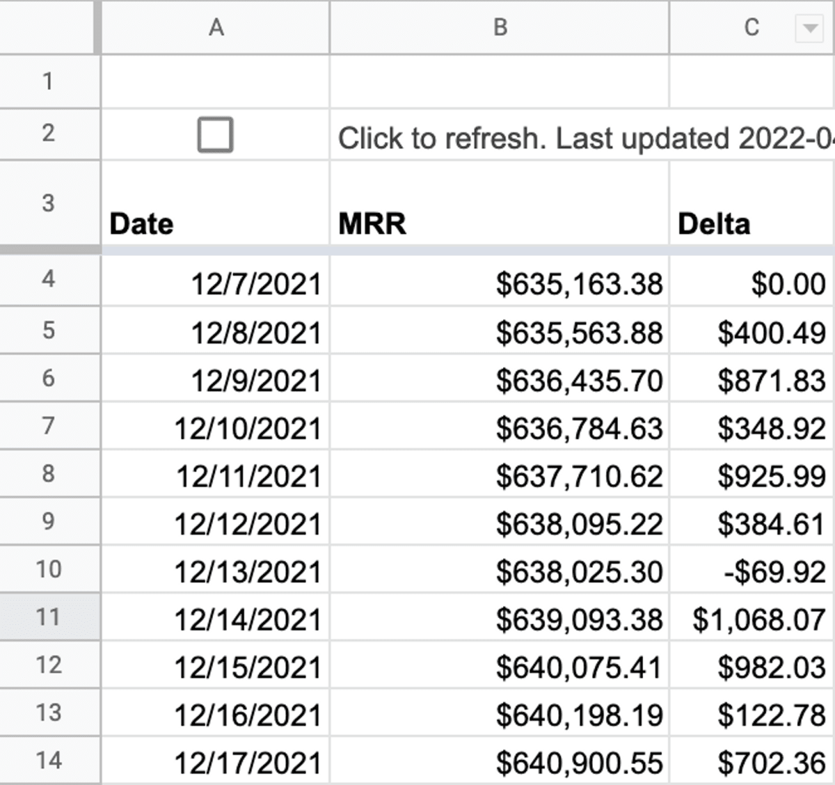
Let’s suppose we are pulling our Daily MRR from Stripe API into Google Sheets and we want to understand how much progress we make each day in terms of adding new MRR and what are trends are for adding incremental MRR each day. The first thing we need to do is add a column showing us the detla of new revenue added each day.

To do this we can use an arrayformula arrayformula(if(B4:B="",,B4:B-{B4;B4:B})), what this does is subtract the current day from the previous day, for the first entry it subtracts it by itself since we don’t know what the previous MRR was. Breaking it down
- The if statement ensures we only do the calculation on items that are not blank =””
- B4:B is all of our daily deltas which we must subtract with an offset
- We add the B4 to the beginning of the array {b4:b4:b} such that when we subtract the arrays they are now offset by 1 and thus we subtract the current day from the previous day to get the delta
Calculating Daily Moving Average
The daily moving average is the set of simple moving averages for all the days in the set of data.
To calculate the simple moving average for a given day we add up all the numbers over the time period and divide by the number of days (arithmetic mean over the time period).
You do this for every day and then you get a time series where the number on a given day is the average of the previous x days which smooths out the value on a given day because it’s just the average of the previous period.
Common periods you might use:
- 7 day to smooth out variances based on the day of the week - eg as a SaaS business focused on business users weekends are slower for us
- 30 day to smooth out monthly aberrations
- 24 hour to smooth out time of day aberrations
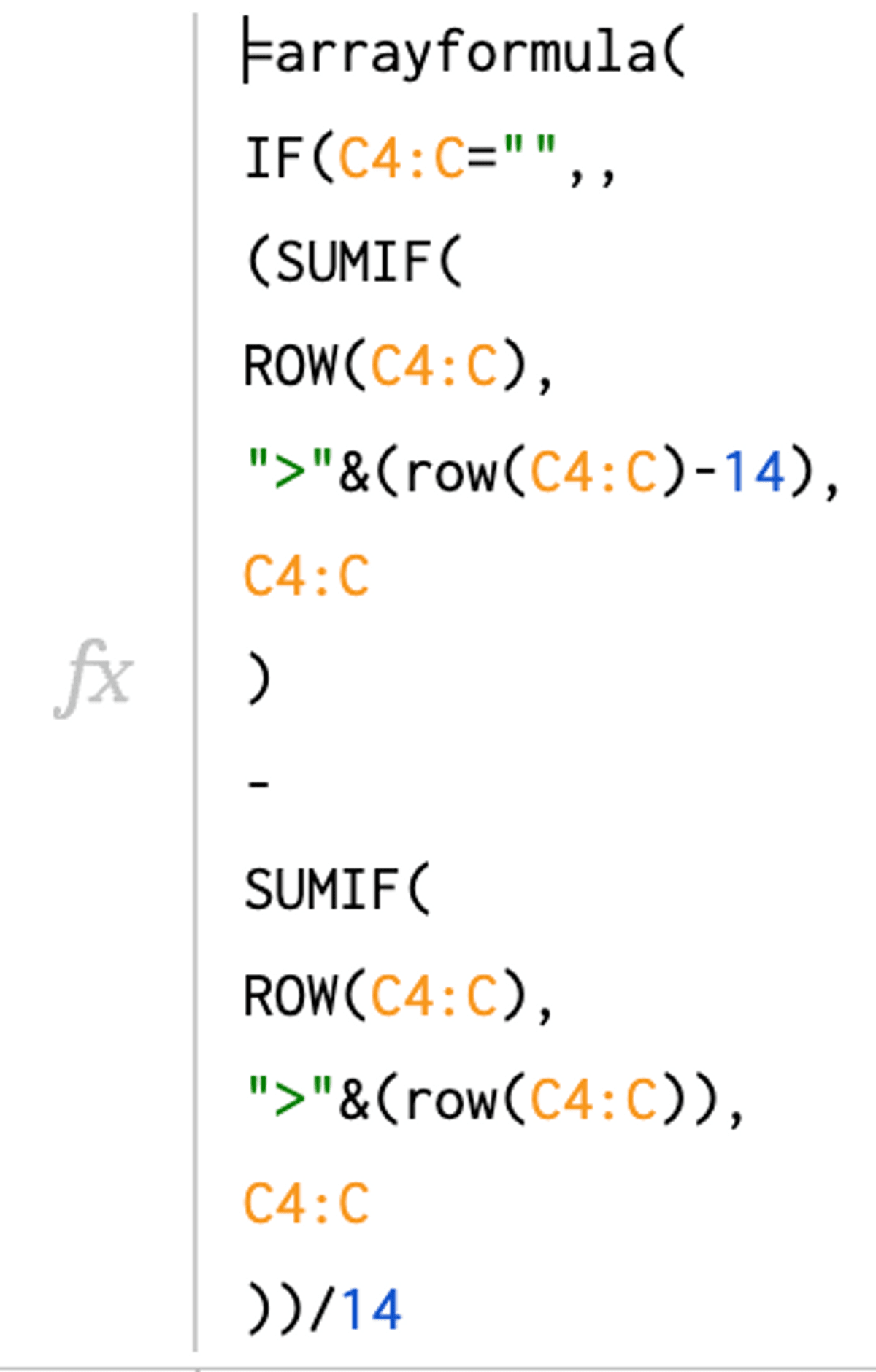
So how to do this with an ARRAY FORMULA in Google Sheets? Using SumIFs. One of the annoying things about Sheets is many of the formulas are not available as array operations, so you have to get creative with the formulas that are available. But the concept is this: A single formula to calculate the moving average for every row in a column.
How to
- For every row get and the date it represents get the sum of all delta mrr greater than 14 days old:
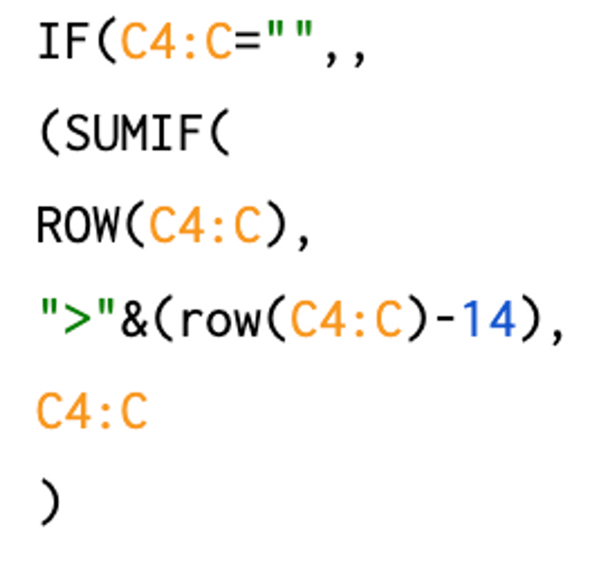
- Only for rows that are blank IF(C4:C="",,
- Make the SUMIF statement evaluate multiple times by making the condition statement have a range (array) in it ">"&(row(C4:C)-14)
- So look at all rows nunbers in column CSUMIF(**ROW(C4:C)** to see if their row number is greater than the current row number - 14 ">"&(row(C4:C)-14)
- C4:C is the delta MRR that gets summed
- So this means for row 16 we look at rows 3→∞ and we sum all their values, then for row 17 we sum all rows from4→∞, and so on and so forth
- It’s certainly a mind bender thinking about how SUMIF works with arrays, so you might want to read it through again, just remember
- SUMIF( rows to compare that never change, condition that runs multiple times, rows to be summed)
- So a condition of row(c4:c)>14 and rows to compare of row(c4:c), and values to sum of c4:c
- so now for every row c4:c we have the MRR deltas that are > 14 days ago for the given row, but we don’t want that we only want >14 days up until the date (row) in question
- So if for every row (date) we subtract the sum of all the rows that are later in date (later rows) then all we’ll be left with is the last 13 days plus the row in question.
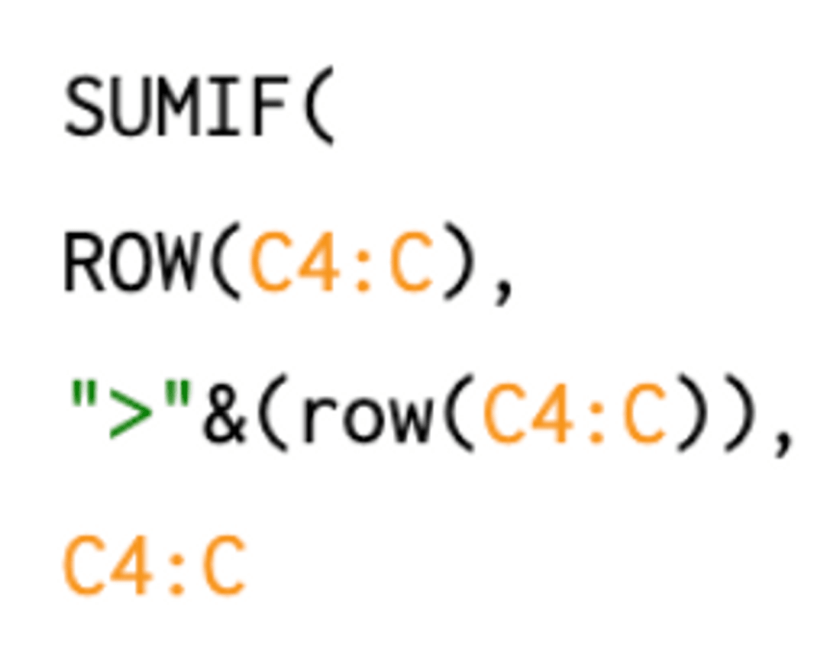
- Get every row sum all the delta mrr that occur after that row. Eg for all delta mrr after a given date sum it up.
- For every row number ROW(c4:C)
- Filter only the rows numbers that are greater than the current row number ">"&(row(C4:C))
- The third parameter of sumif lets us set a seperate column to sum, so we sum the actual values of `C4:C` (which are the delta MRRs)
- We now have an array where every row in it is the sum of that dates mrr delta as well as the proceeding 13 days - 14 days of MRR Delta. We then divide every row by 14 and we now have an array where every row is a day and the value in it is the mean of the 14 days of MRR delta
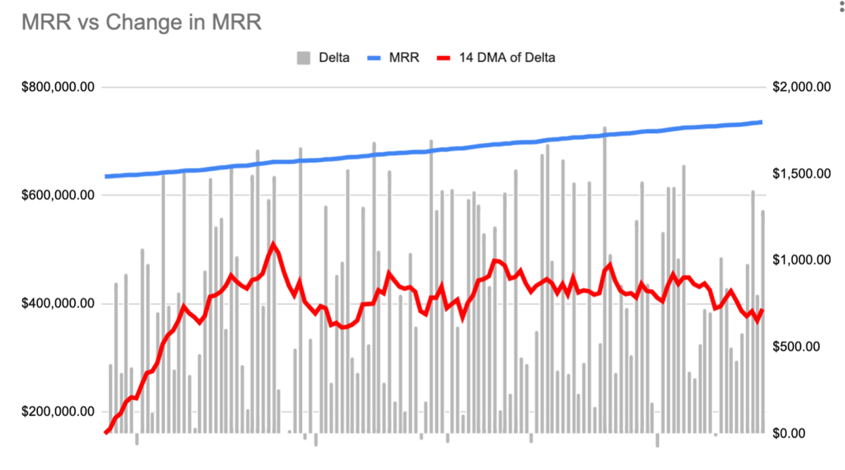
Now we can graph our MRR over time with the MRR delta and the MRR Delta 14 DMA:
- We can see our MRR rising
- We can see that our MRR change per day is quite noise
- We can see that our 14DMA of the MRR delta is pretty flat meaning we’re not accelerating our growth in MRR, we’re only growing linearly